- [RQ1]The team's first mission is to develop a deep understanding of waste generation patterns during the normal period as well as to find out the relationship between socioeconomic background and waste generation. Based on that, the team could predict the volume of waste generation to make a proper business model and give suggestions.
- [RQ2]The second mission of the team is to explore how the normal waste generation pattern changed during the Covid-19 period on the geographical aspect and how socioeconomic factors play its role at this time. By digging deeper into pattern changes in both COVID-19 periods, the team implemented those insights into our business model and recommendations.
- [H1] The team supposed the waste generation pattern in the normal period steadily fluctuates over the years. Community districts with higher median household income will generate more waste than community districts with a lower median household income.
- [H2] During the stay at home period, the team supposed the amount of residential refuse generated would skyrocket due to limited mobility in all five boroughs, paper, and mix recyclable would slightly decline due to more reuse than disposal. Neighborhoods with more residential zonings experienced a more significant increase in waste generation. High-income areas would see less of an increase because residents left the city to avoid pandemic hot zones, while more impoverished neighborhoods would see more of an increase because people can't afford to leave.
DSNY Monthly Tonnage Data
NYC Planning | Community Profiles
- Time Series Analysis The team used the NYC tonnage dataset and focused on the near-term data which were after January 2010. We summed up the data into borough scale while originally the data were in community district scale. Then we applied a basic time series model to visualize the trend of all types of waste generation and how they changed during the last decade. And the team also created a heatmap of correlation between three main waste types.
- Social-Economic Spatial Analysis We merged demographic information with waste data. Then, we generated several heatmaps to visualize waste collection tonnage. Later, the team conducted clustering analysis seeking the relationship between median household income and per capita waste generation among all community districts. After that, the team applied a regression model from the statsmodels module to community district clusters found in the previous clustering result to test the initial hypothesis about waste-demographic correlation and made conclusions.
- Time Series Analysis Regarding the current shock of COVID-19, we built a time series model to get the predicted value during March to June and then compared the prediction with the actual values of waste generation. Considering the large proportion of refuse waste and high correlation among these three wastes, we chose refuse waste as an example and built a time series model for each boro.
- Social-Economic Spatial Analysis The analytical methodology in this section is identical to section 6.1.2. But in this section, the team will use the analysis result to test different sets of hypotheses under the timeframe of Covid-19 NYC Stay At Home order period.
- Suggestions Based on the previous analythese, the team estimated on what kind of waste is causing the most economic losses as well as looked at entities which have been playing important roles in the circular economy, including startups, academic institutions, venture capitals to help reduce the economic losses of waste. After that, the team also came up with related suggestions and a potential business model to give a more straightforward explanation.
General Waste Analysis
1. Time Series Analysis
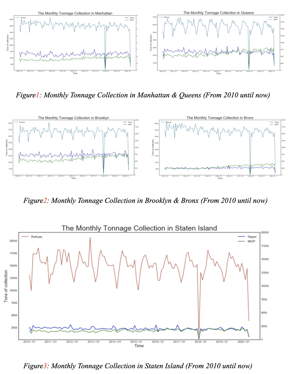
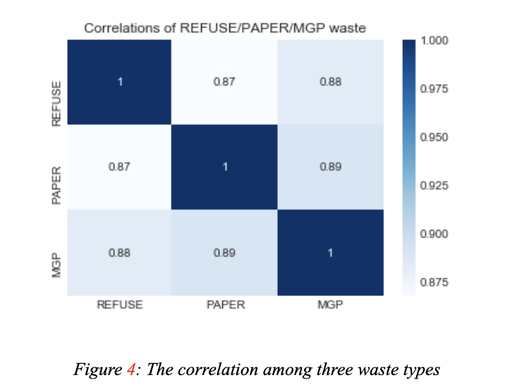
From the visualizations in Figure 1-3, we can see that Refuse waste occupies the largest proportion in all wastes. There is also seasonality in all five boroughs while there isn’t any obvious trend in these time series data. People tend to generate more waste during summer time than winter time. Moreover, due to the same-direction change of all these three types of wastes shown in the above visualization, there are high correlations (Figure 4) among the three types, which can also simplify our previous model of time series
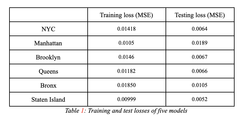
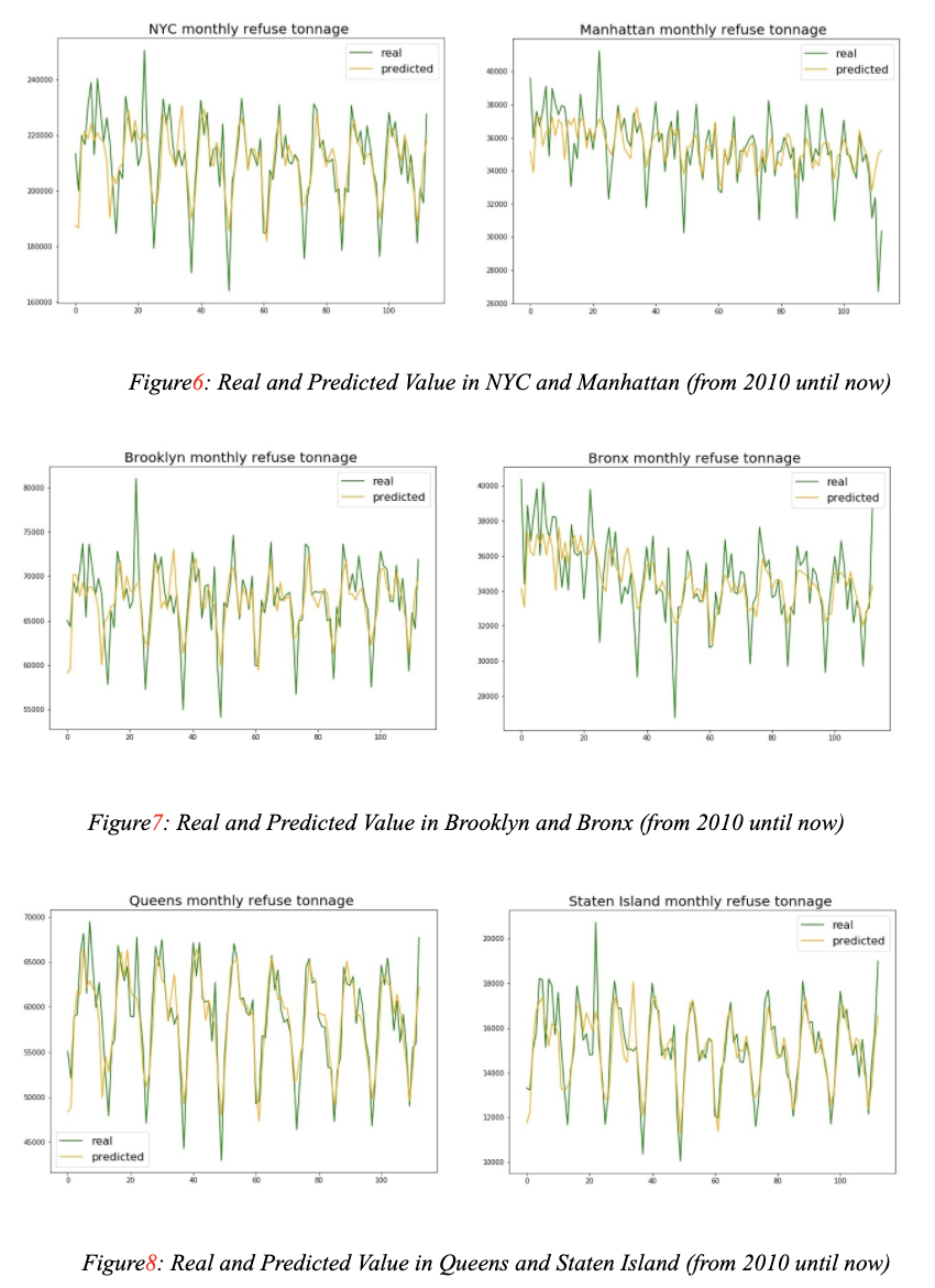
The results of the six time series models mentioned in par are shown in Table 1. The real and predicted values are shown in Figure 6-8.
As we can see above, LSTM structure has captured the fluctuation of the time series successfully. All the five boros have similar trends as well as seasonality. The waste generation reached its maximum during the summer time while in winter it reduced to its lowest point. This pattern may suggest different manipulation on waste and circular economy in different seasons.
2. Analysis on DSNY tonnage collection in space(2015-2019)
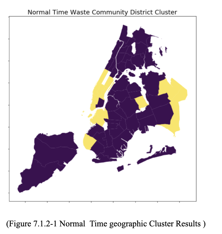
In the clustering analysis, the silhouette-score from Gaussian Mixture equals 0.3988. The algorithm provided two clusters that it calculated to have relations, Figure 7.1.2-1 is a geographic representation of the two clusters.
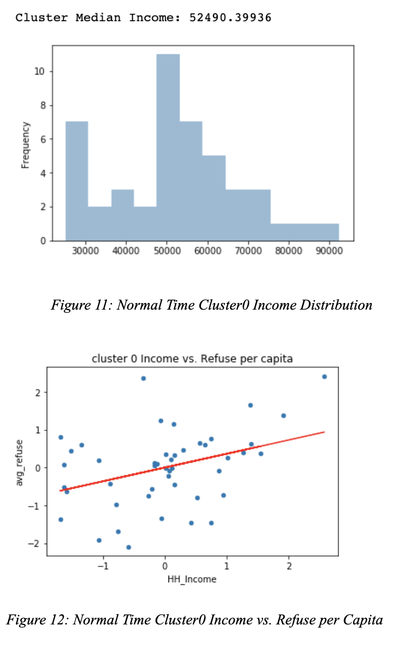
the first cluster(dark blue) contained most of the community districts that has lower household income, and the median household income in this cluster was $52,490 , and most of the community districts distributed in the 50k-65k range. (figure 11 in appendix).
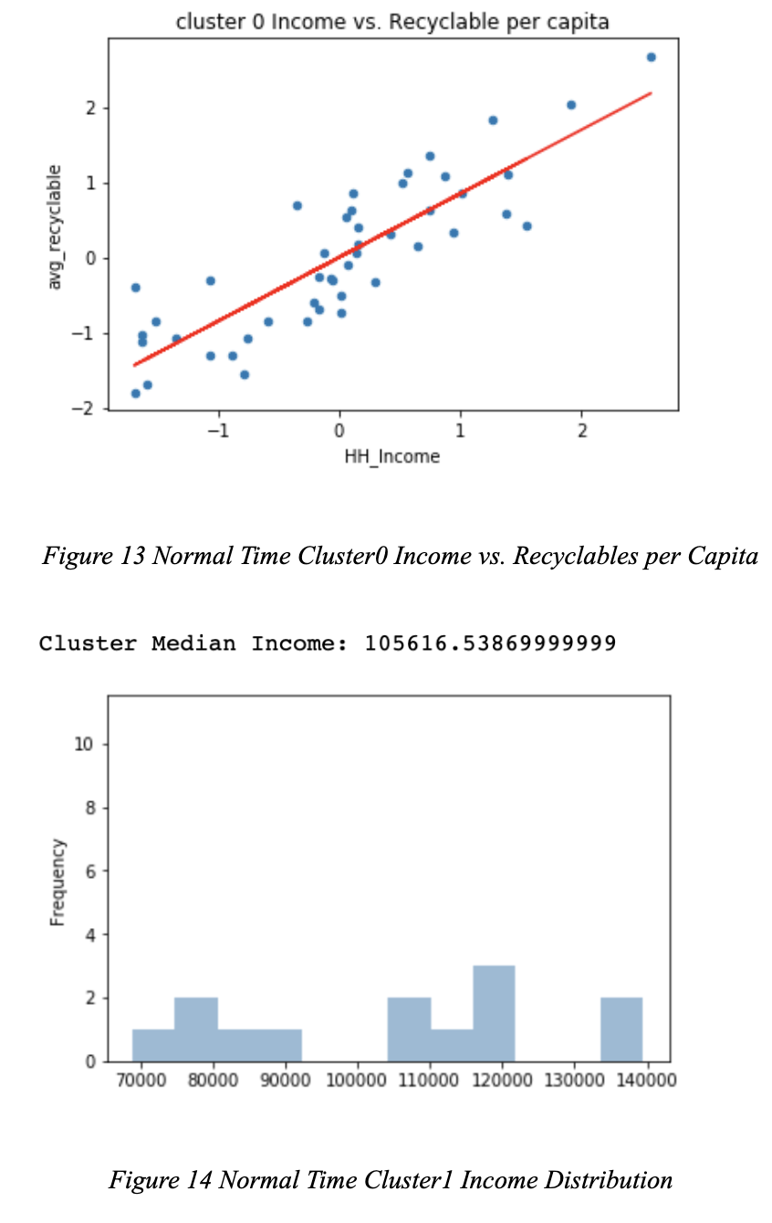
After applying regression model to this cluster, the result shows that there was a positive correlation between income and refuse generation per capita (figure 12 in appendix) with coefficient=0.3964, and positive correlation between income and recyclable (paper + mix-recyclable) generation per capita (figure 13) with coefficient=0.8617. The second cluster (light yellow) contained most of the community districts that had higher household income and the median household income in this cluster was $105,616 (Figure 14).
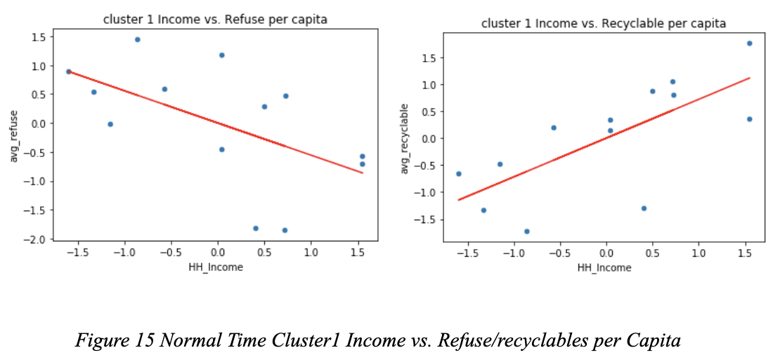
The result of regression analysis showed differences between the second and the first cluster. There was a negative correlation between income and refuse generation per capita (Figure 15 in appendix) with coefficient=-0.557; and positive correlation between income and recyclable (paper + mix-recyclable) generation per capita (figure 15) with coefficient=0.7175.
From the above analysis result, we can conclude that Income does affect waste generation. In the lower income cluster, with the rise of household income, refuse generation per capita increases in tandem, so does recyclables (paper+mix-recyclables) generation per capita. But in the higher income cluster, refuse generation per capita decreases while household income rises even though the tandem of recyclables generation remains positive while income increases. In short, social economic background has different influences across various income levels, especially in refuse generation, but not much influences on recyclables generation.
Covid-19 Waste Analysis
1. Time Series Prediction
Based on our time series model, it can be seen that all the boroughs except Manhattan had a surge in waste generation in COVID-19 periods, especially in June. This may be partly explained by the fact that people who lived outside Manhattan didn’t have to go to Manhattan for work during stay-at-home policy.
2. Analysis on DSNY tonnage collection in space(Stay At Home Period ~ March-June)
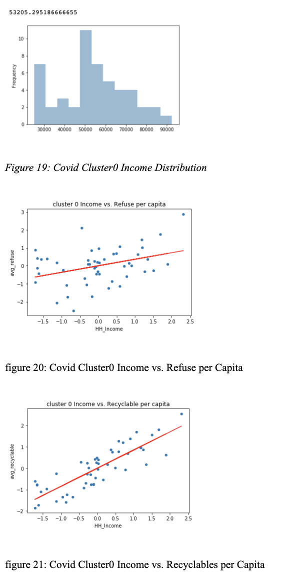
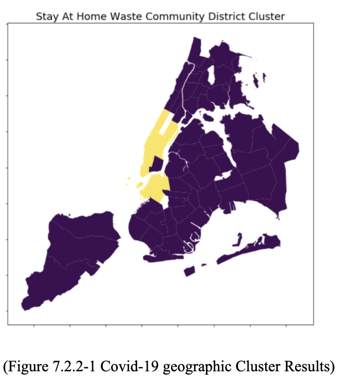
We applied the same concept as we used in section 7.1.2, Gaussian Mixture clustering with silhouette-score equals 0.4702. The algorithm provided two clusters that it calculated to have relations, figure 7.2.2-1 is a geographic representation of the two clusters, In the first cluster(dark blue), it contained community districts that had median households as $53,205, and most of the community districts distributed in the 50k-65k range. (figure 19)
The result of regression model shows that there was a moderate positive correlation between income and refuse generation per capita (figure 20) with coefficient=0.3638, and strong positive correlation between income and recyclable (paper + mix-recyclable) generation per capita (figure 21) with coefficient=0.8469.
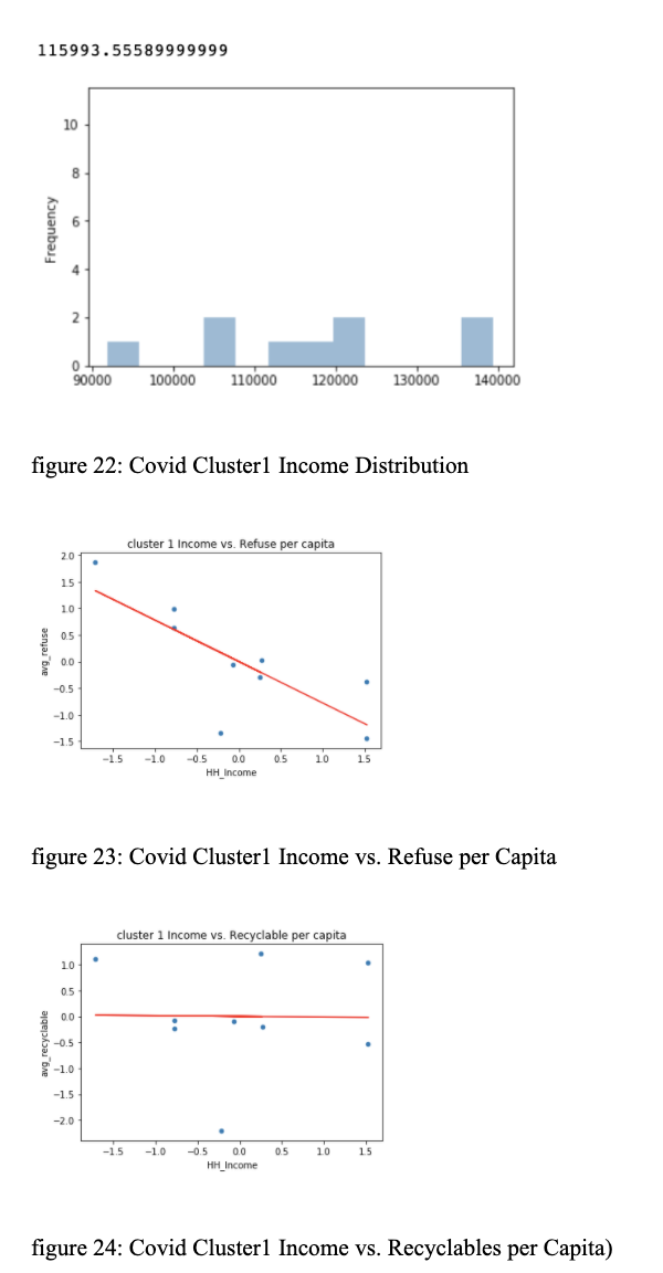
The second cluster (light yellow) contained most of the community districts that had higher household income and the median household income in this cluster was $115,993 (figure 22).
The result of regression showed there was a strong negative correlation between income and refuse generation per capita (figure 23) with coefficient=-0.7784, and very weak negative correlation between income and recyclable (paper + mix-recyclable) generation per capita (figure 24 in appendix) with coefficient=-0.0136.